from https://github.com/grantmcdermott/parttree
Installation
This package is not yet on CRAN, but can be installed from GitHub with:
# install.packages("remotes")
remotes::install_github("grantmcdermott/parttree")
Example
The main function that users will interact with is geom_parttree(). Here’s a simple example.
library(parttree)
library(rpart)
library(ggplot2)

iris_tree = rpart(Species ~ Sepal.Width + Petal.Width, data=iris)

## Let's construct a scatterplot of the original iris data
p = ggplot(data = iris, aes(x=Petal.Width, y=Sepal.Width)) +
  geom_point(aes(col=Species))

## We now add the partitions with geom_parttree()
p +
  geom_parttree(data = iris_tree, aes(fill=Species), alpha = 0.1) +
  labs(caption = "Note: Points denote observed data. Shaded regions denote tree predictions.")

Limitations and caveats
Supported model classes
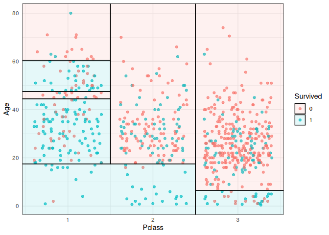
Currently, the package only works with decision trees created by the rpart package. However, it does support other packages and modes that call rpart::rpart() as the underlying engine. Here’s an example using the parsnip package.
library(parsnip)
library(titanic) ## Just for a different data set
set.seed(123) ## For consistent jitter

titanic_train$Survived = as.factor(titanic_train$Survived)

## Build our tree using parsnip (but with rpart as the model engine)
ti_tree =
  decision_tree() %>%
  set_engine("rpart") %>%
  set_mode("classification") %>%
  fit(Survived ~ Pclass + Age, data = titanic_train)

## Plot the data and model partitions
titanic_train %>%
  ggplot(aes(x=Pclass, y=Age)) +
  geom_jitter(aes(col=Survived), alpha=0.7) +
  geom_parttree(data = ti_tree, aes(fill=Survived), alpha = 0.1) +
  theme_minimal()
#> Warning: Removed 177 rows containing missing values (geom_point).
Orientation
Underneath the hood, geom_parttree() is calling the companion parttree() function, which coerces the rpart tree object into a data frame that is easily understood by ggplot2. For example, consider our “ti_tree” model from above. Here’s the print output of the raw model.
ti_tree
#> parsnip model object
#>
#> Fit time:  6ms
#> n= 891
#>
#> node), split, n, loss, yval, (yprob)
#>       * denotes terminal node
#>
#>   1) root 891 342 0 (0.61616162 0.38383838)
#>     2) Pclass>=2.5 491 119 0 (0.75763747 0.24236253)
#>       4) Age>=6.5 461 102 0 (0.77874187 0.22125813) *
#>       5) Age< 6.5 30  13 1 (0.43333333 0.56666667) *
#>     3) Pclass< 2.5 400 177 1 (0.44250000 0.55750000)
#>       6) Age>=17.5 365 174 1 (0.47671233 0.52328767)
#>        12) Pclass>=1.5 161  66 0 (0.59006211 0.40993789) *
#>        13) Pclass< 1.5 204  79 1 (0.38725490 0.61274510)
#>          26) Age>=44.5 67  32 0 (0.52238806 0.47761194)
#>            52) Age>=60.5 14   3 0 (0.78571429 0.21428571) *
#>            53) Age< 60.5 53  24 1 (0.45283019 0.54716981)
#>             106) Age< 47.5 13   3 0 (0.76923077 0.23076923) *
#>             107) Age>=47.5 40  14 1 (0.35000000 0.65000000) *
#>          27) Age< 44.5 137  44 1 (0.32116788 0.67883212) *
#>       7) Age< 17.5 35   3 1 (0.08571429 0.91428571) *
And here’s what we get after we feed it to parttree().
parttree(ti_tree)
#>   node Survived
#> 1    4        0
#> 2    5        1
#> 3    7        1
#> 4   12        0
#> 5   27        1
#> 6   52        0
#> 7  106        0
#> 8  107        1
#>                                                                                              path
#> 1                                                                    Pclass >= 2.5 --> Age >= 6.5
#> 2                                                                    Pclass >= 2.5 --> Age <  6.5
#> 3                                                                   Pclass <  2.5 --> Age <  17.5
#> 4                                                 Pclass <  2.5 --> Age >= 17.5 --> Pclass >= 1.5
#> 5                                 Pclass <  2.5 --> Age >= 17.5 --> Pclass <  1.5 --> Age <  44.5
#> 6                 Pclass <  2.5 --> Age >= 17.5 --> Pclass <  1.5 --> Age >= 44.5 --> Age >= 60.5
#> 7 Pclass <  2.5 --> Age >= 17.5 --> Pclass <  1.5 --> Age >= 44.5 --> Age <  60.5 --> Age <  47.5
#> 8 Pclass <  2.5 --> Age >= 17.5 --> Pclass <  1.5 --> Age >= 44.5 --> Age <  60.5 --> Age >= 47.5
#>   xmin xmax ymin ymax
#> 1  2.5  Inf  6.5  Inf
#> 2  2.5  Inf -Inf  6.5
#> 3 -Inf  2.5 -Inf 17.5
#> 4  1.5  2.5 17.5  Inf
#> 5 -Inf  1.5 17.5 44.5
#> 6 -Inf  1.5 60.5  Inf
#> 7 -Inf  1.5 44.5 47.5
#> 8 -Inf  1.5 47.5 60.5
Again, the resulting data frame is designed to be amenable to a ggplot2 geom layer, with columns like xmin, xmax, etc. specifying aesthetics that ggplot2 recognises. (Fun fact: geom_partree() is really just a thin wrapper around geom_rect().) The goal of the package is to abstract away these kinds of details from the user, so we can just specify geom_parttree() — with a valid tree object as the data input — and be done with it. However, while this generally works well, it can sometimes lead to unexpected behaviour in terms of plot orientation. That’s because it’s hard to guess ahead of time what the user will specify as the x and y axes/variables in their other plot layers. To see what I mean, let’s redo our titanic plot from earlier, but this time switch the axes in the main ggplot() call.
titanic_train %>%
  ggplot(aes(x=Age, y=Pclass)) + ## Changed!
  geom_jitter(aes(col=Survived), alpha=0.7) +
  geom_parttree(data = ti_tree, aes(fill=Survived), alpha = 0.1) +
  theme_minimal() +
  labs(title = "Oops!")
#> Warning: Removed 177 rows containing missing values (geom_point).
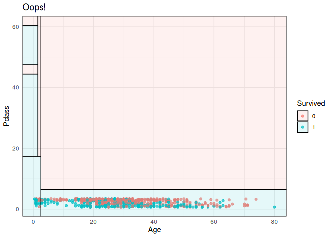
Normally, this kind of orientation mismatch should be pretty easy to recognize (as is the case here). But its admittedly annoying. I’ll try to add better support for catching/avoiding these kinds of errors in a future update, but as of the moment: caveat emptor.