SOM分析基本理论
SOM (Self-Organizing Feature Map,自组织特征图)是基于神经网络方式的数据矩阵和可视化方式。与其它类型的中心点聚类算法如K-means等相似,SOM也是找到一组中心点 (又称为codebook vector),然后根据最相似原则把数据集的每个对象映射到对应的中心点。在神经网络术语中,每个神经元对应于一个中心点。
与K-means类似,数据集中的每个对象每次处理一个,判断最近的中心点,然后更新中心点。与K-means不同的是,SOM中中心点之间存在拓扑形状顺序,在更新一个中心点的同时,邻近的中心点也会随着更新,直到达到设定的阈值或中心点不再有显著变化。最终获得一系列的中心点 (codes)隐式地定义多个簇,与这个中心点最近的对象归为同一个簇。
SOM强调簇中心点之间的邻近关系,相邻的簇之间相关性更强,更有利于解释结果,常用于可视化网络数据或基因表达数据。
Even though SOM is similar to K-means, there is a fundamental difference. Centroids used in SOM have a predetermined topographic ordering relationship. During the training process, SOM uses each data point to update the closest centroid and centroids that are nearby in the topographic ordering. In this way, SOM produces an ordered set of centroids for any given data set. In other words, the centroids that are close to each other in the SOM grid are more closely related to each other than to the centroids that are farther away. Because of this constraint, the centroids of a two-dimensional SOM can be viewed as lying on a two-dimensional surface that tries to fit the n-dimensional data as well as possible. The SOM centroids can also be thought of as the result of a nonlinear regression with respect to the data points. At a high level, clustering using the SOM technique consists of the steps described in Algorithm below:
1: Initialize the centroids.
3: Select the next object.
4: Determine the closest centroid to the object.
5: Update this centroid and the centroids that are close, i.e., in a specified neighborhood.
6: until The centroids don‘t change much or a threshold is exceeded.
7: Assign each object to its closest centroid and return the centroids and clusters.
SOM分析实战
下面是R中用kohonen包进行基因表达数据的SOM分析。
加载或安装包
读入数据并进行标准化
data <- read.table(“ehbio_trans.Count_matrix.xls”, row.names=1, header=T, sep=“t”)
data_train_matrix <- as.matrix(t(scale(t(data))))
names(data_train_matrix) <- names(data)
untrt_N61311 untrt_N052611 untrt_N080611 untrt_N061011 trt_N61311
ENSG00000223972 1.6201852 -0.5400617 -0.5400617 -0.5400617 -0.5400617
ENSG00000227232 -1.0711639 1.0274429 0.6776751 0.8525590 -1.2460478
ENSG00000278267 -1.6476479 1.3480756 0.1497862 0.7489309 -0.4493585
ENSG00000237613 2.4748737 -0.3535534 -0.3535534 -0.3535534 -0.3535534
ENSG00000238009 -0.3535534 -0.3535534 -0.3535534 -0.3535534 2.4748737
ENSG00000268903 -0.7020086 0.9025825 -0.7020086 -0.7020086 -0.7020086
trt_N052611 trt_N080611 trt_N061011
ENSG00000223972 1.6201852 -0.5400617 -0.5400617
ENSG00000227232 -1.2460478 0.5027912 0.5027912
ENSG00000278267 0.7489309 0.1497862 -1.0485032
ENSG00000237613 -0.3535534 -0.3535534 -0.3535534
ENSG00000238009 -0.3535534 -0.3535534 -0.3535534
ENSG00000268903 0.9025825 -0.7020086 1.7048781
训练SOM模型
som_grid <- somgrid(xdim = 10, ydim=10, topo=“hexagonal”)
som_model <- supersom(data_train_matrix, grid=som_grid, keep.data = TRUE)
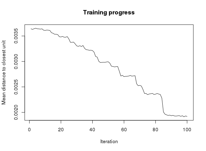
可视化SOM结果
plot(som_model, type = “changes”)
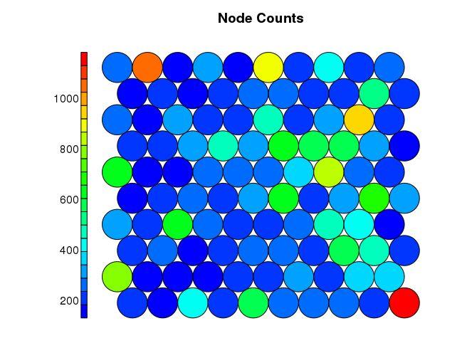
计量每个SOM中心点包含的基因的数目
coolBlueHotRed <- function(n, alpha = 0.7) {
rainbow(n, end=4/6, alpha=alpha)[n:1]
plot(som_model, type = “counts”, main=“Node Counts”, palette.name=coolBlueHotRed)
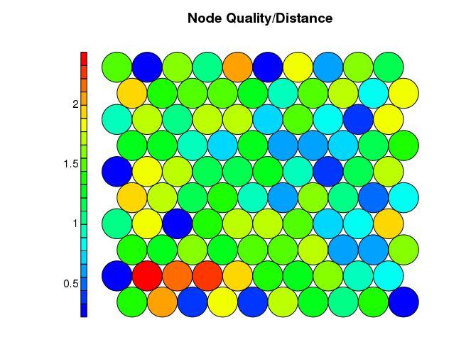
计量SOM中心点的内敛性和质量
plot(som_model, type = “quality”, main=“Node Quality/Distance”, palette.name=coolBlueHotRed)
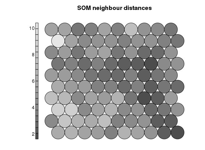
邻居距离-查看潜在边界点
plot(som_model, type=“dist.neighbours”, main = “SOM neighbour distances”, palette.name=grey.colors)
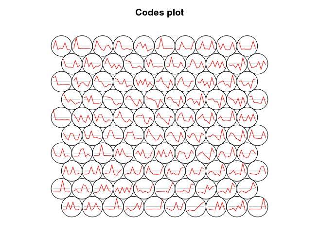
查看SOM中心点的变化趋势
plot(som_model, type = “codes”, codeRendering=“lines”)
获取每个SOM中心点相关的基因
table(som_model$unit.classif)
som_model_code_class = data.frame(name=rownames(data_train_matrix), code_class=som_model$unit.classif)
head(som_model_code_class)
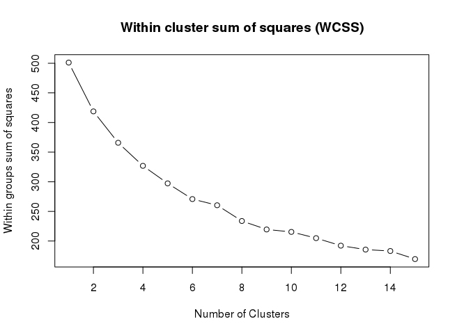
SOM结果进一步聚类
mydata <- as.matrix(as.data.frame(som_model$codes))
wss <- (nrow(mydata)-1)*sum(apply(mydata,2,var))
for (i in 2:15) wss[i] <- sum(kmeans(mydata, centers=i)$withinss)
par(mar=c(5.1,4.1,4.1,2.1))
plot(1:15, wss, type=“b”, xlab=“Number of Clusters”,
ylab=“Within groups sum of squares”, main=“Within cluster sum of squares (WCSS)”)
som_cluster <- cutree(hclust(dist(mydata)), 6)
cluster_palette <- function(x, alpha = 0.6) {
n = length(unique(x)) * 2
rainbow(n, start=2/6, end=6/6, alpha=alpha)[seq(n,0,-2)]
cluster_palette_init = cluster_palette(som_cluster)
bgcol = cluster_palette_init[som_cluster]
plot(som_model, type=“codes”, bgcol = bgcol, main = “Clusters”, codeRendering=“lines”)
add.cluster.boundaries(som_model, som_cluster)
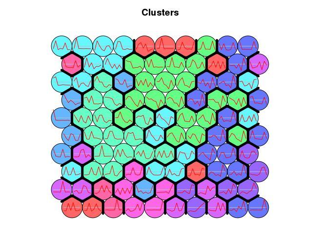
有一些类的模式不太明显,以后再看怎么优化。
SOM获取基因所在的新类
som_model_code_class_cluster = som_model_code_class
som_model_code_class_cluster$cluster = som_cluster[som_model_code_class$code_class]
head(som_model_code_class_cluster)
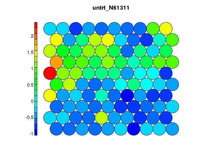
映射某个属性到SOM图
color_by_var = names(data_train_matrix)[1]
color_by = data_train_matrix[,color_by_var]
unit_colors <- aggregate(color_by, by=list(som_model$unit.classif), FUN=mean, simplify=TRUE)
plot(som_model, type = “property”, property=unit_colors[,2], main=color_by_var, palette.name=coolBlueHotRed)